SEC/GPC Theory Series Part 2: Calibration Theory, Molecular Weight and Universal Calibration

Updated: Jul 23
This article forms Part 2 of the Chromperfect SEC/GPC Theory Series, created to provide a structured and detailed explanation of the principles behind size exclusion chromatography and gel permeation chromatography.
Part 1 examines SEC integration theory, including the dedicated SEC baseline, detector noise, internal-standard flow correction, detector-response types, molecular-weight averages and molecular-weight fractions.
This second article focuses on SEC calibration theory, including the physical meaning of molecular-weight averages, SEC calibration curves, narrow-standard calibration, universal calibration, intrinsic viscosity, hydrodynamic volume and broad-standard calibration methods.
Part 3 completes the series by examining advanced SEC concepts, including molecular-weight-distribution plots, axial broadening, axial correction, calculated molecular-weight traces, local polydispersity and preparative fractionation.
This article accompanies our video, “The Complete Guide to SEC Calibration Theory | GPC & Molecular Weight,” which provides a detailed technical explanation of the calibration principles discussed below.
This article summarizes the principal subjects covered in the video. Because the video is an in-depth technical presentation, the article should be treated as a structured overview rather than a complete replacement for the full explanation. For the most detailed discussion of the equations, assumptions, limitations and differences between SEC calibration methods, watch the complete video.
The presentation follows the SEC calibration theory described in the Chromperfect documentation and covers the route from chromatographic elution data to defensible molecular-weight information.
What is SEC calibration?
Size exclusion chromatography, commonly abbreviated as SEC, separates dissolved molecules primarily according to their effective size in solution. In polymer analysis, SEC is also widely known as gel permeation chromatography, or GPC.
An SEC chromatogram initially records detector response as a function of elution time or elution volume. On its own, this chromatographic response does not directly identify the molecular weight of the material passing through the detector.
An SEC calibration curve provides the relationship required to convert chromatographic position into:
Molecular weight
Molecular size
Hydrodynamic volume
A calculated molecular-weight distribution
The calibration relationship is therefore the bridge between the chromatogram and the molecular-weight results reported for a polymer sample.

A reliable SEC calibration is more than a mathematical curve fitted through several points. It represents a physical relationship between the behaviour of molecules in the SEC column and their effective size under defined analytical conditions.
Those conditions may include:
The polymer type
The solvent
The column or column set
The flow rate
The operating temperature
The detector response
The calibration-standard data
The selected calibration model
The purpose of SEC calibration theory is to understand how these factors affect the conversion from elution position to molecular weight.
Why polymers require molecular-weight averages - SEC calibration theory
Many ordinary chemical compounds consist of molecules with one defined molecular weight. A pure low-molecular-weight compound can therefore be described using a single molecular formula and a single molecular weight.
Polymers are often different.
During polymerization, individual polymer chains may stop growing at different stages. As a result, a synthetic polymer sample commonly contains chains with different numbers of repeating units and therefore different molecular weights.
A polymer containing molecules of many molecular weights is described as polydisperse. A material in which all molecules have the same molecular weight is described as monodisperse.

Because a polydisperse polymer does not have one uniquely defined molecular weight, it must be described using a series of molecular-weight averages. Each average gives a different statistical weighting to the molecules within the distribution.
The principal molecular-weight averages discussed in SEC and GPC include:
Number-average molecular weight, Mn
Viscosity-average molecular weight, Mv
Weight-average molecular weight, Mw
Z-average molecular weight, Mz
Z-plus-one average molecular weight, Mz+1
Chromperfect calculates these molecular-weight averages from the processed SEC distribution, together with related molecular-weight fractions and intrinsic-viscosity information where the required constants are available.
Number-average molecular weight, Mn
The number-average molecular weight, Mn, gives every molecule equal statistical importance.
A small molecule counts once, and a large molecule also counts once. The molecular weights of all molecules are added together and divided by the total number of molecules.
The general expression is:
Mn = Σ(Ni × Mi) / ΣNi
where:
Ni is the number of molecules having molecular weight Mi
Mi is the molecular weight of that group of molecules
Because every molecule contributes equally to the molecule count, Mn is strongly influenced by the low-molecular-weight portion of the distribution.
Number-average molecular weight is commonly associated with measurements that depend primarily on the number of dissolved particles, such as osmotic-pressure measurements. It may also be related to properties affected by the number of polymer chain ends.

Weight-average molecular weight, Mw
The weight-average molecular weight, Mw, gives greater statistical importance to larger molecules.
Its general expression is:
Mw = Σ(Ni × Mi²) / Σ(Ni × Mi)
Because molecular weight is squared in the numerator, large polymer chains make a stronger contribution to Mw than small chains.
This means that Mw is normally higher than Mn for a polydisperse polymer. Weight-average molecular weight is often associated with large-angle light-scattering measurements and may relate more closely than Mn to properties dominated by larger chains.

Z-average, Z-plus-one and viscosity-average molecular weight
The Z-average molecular weight, Mz, applies an even stronger weighting to the high-molecular-weight region of the distribution.
The Z-plus-one average, Mz+1, increases that high-molecular-weight emphasis still further. These higher-order averages are particularly sensitive to the largest molecules and to the high-molecular-weight tail of a polymer distribution.
The viscosity-average molecular weight, Mv, is different because it is linked to the effect of the polymer on solution viscosity. Its value depends on the polymer, solvent, temperature and Mark–Houwink exponent.
For a typical polydisperse polymer, the molecular-weight averages usually follow the approximate order:
Mn ≤ Mv ≤ Mw ≤ Mz ≤ Mz+1
The precise position of Mv depends on the Mark–Houwink exponent, α.

Dispersity and molecular-weight-distribution breadth
The difference between Mn and Mw provides useful information about the breadth of a molecular-weight distribution.
The most common measure is dispersity, represented by:
Đ = Mw / Mn
Dispersity has also traditionally been called the polydispersity index.
For an ideal monodisperse material:
Mw = Mn
and therefore:
Đ = 1
For a polydisperse material, Mw is greater than Mn, so dispersity is greater than one.
A correctly calculated non-negative molecular-weight distribution cannot produce a dispersity below one.
A larger dispersity normally indicates a broader molecular-weight distribution, but a broad distribution is not necessarily undesirable. The appropriate molecular-weight profile depends on the intended material, manufacturing process and application.

General properties of an SEC calibration curve
An SEC calibration curve connects elution position with a molecular-weight-related value.
The horizontal axis normally represents:
Elution time, or
Elution volume
The vertical axis commonly represents:
Logarithmic molecular weight, or
Logarithmic hydrodynamic volume for universal calibration
Strictly speaking, SEC separates molecules according to elution volume. However, when flow rate is stable, elution time is proportional to elution volume:
Ve = F × te
where:
Ve is elution volume
F is flow rate
te is elution time
Stable flow is therefore essential when an SEC calibration is expressed in time units.
Why SEC calibration uses logarithmic molecular weight
An SEC separation may cover several decades of molecular weight. For example, a column set might separate material ranging from approximately 10³ to 10⁶ in molecular weight.
On a linear molecular-weight axis, the lower decades would be compressed into a very small portion of the scale. Plotting the logarithm of molecular weight gives each decade equal graphical space.
This creates a more practical relationship between molecular weight and elution volume.

Why large molecules elute before small molecules in SEC
SEC columns contain porous particles.
Large molecules cannot enter as many pores and therefore travel through a smaller proportion of the stationary-phase pore volume. Their effective path through the column is shorter, so they elute earlier.
Small molecules can enter more of the accessible pores. They follow a longer path and elute later.
Consequently, a conventional SEC molecular-weight calibration curve slopes downward:
Early elution corresponds to larger molecular size and higher molecular weight
Late elution corresponds to smaller molecular size and lower molecular weight

Fully excluded and fully included regions
Every SEC column has an upper and lower useful separation limit.
Fully excluded molecules
Molecules above the upper separation limit are too large to enter a significant proportion of the pores. They are fully excluded and tend to elute together near the exclusion volume, V0.
The column cannot distinguish effectively between molecular sizes above this upper limit.
Fully included molecules
Molecules below the lower separation limit are small enough to enter essentially all accessible pores. They are fully included and tend to elute near the total permeation volume, Vt.
Below this limit, the column again loses the ability to discriminate according to molecular size.
The useful SEC calibration range lies between these fully excluded and fully included regions.

Linear and polynomial SEC calibration curves
A plot of log molecular weight against elution time or elution volume may be approximately linear through part of the working range. However, an SEC calibration curve is not necessarily linear across the complete separation range.
Curvature may occur:
Near the upper or lower separation limits
When the column set contains a complex distribution of pore sizes
When several columns with different exclusion ranges are combined
For this reason, Chromperfect supports polynomial SEC calibration curves rather than requiring every calibration to be linear.
The selected polynomial degree should be no more complex than the calibration data justify.
A higher-degree polynomial may follow genuine curvature more closely, but it also requires enough reliable, well-distributed calibration points. An unnecessarily high polynomial degree can create unrealistic bends between standards and produce large molecular-weight errors.
Because molecular weight is represented logarithmically, even a visually small error in log molecular weight can correspond to a substantial error in the calculated molecular weight.

Why extrapolation beyond an SEC calibration range is hazardous
Calibration standards should cover the molecular-weight range expected in the samples.
Extrapolation beyond the standard range is particularly hazardous in SEC because:
Molecular weight is logarithmic
A small change in elution position may represent a large change in molecular weight
Polynomial behaviour is unconstrained outside the calibration points
The column may be approaching a region with limited size discrimination
Software may still calculate a value outside the calibrated range, but the existence of a calculated number does not demonstrate that the value is reliable.
Results obtained through extrapolation should therefore be interpreted with caution.

Narrow-standard SEC calibration
The most direct SEC calibration method uses a series of narrow molecular-weight standards.
A narrow standard has a molecular-weight distribution sufficiently narrow that its molecular-weight averages can be treated as approximately equal for calibration purposes:
Mn ≈ Mw ≈ Mz
Each standard is analyzed under the intended chromatographic conditions. The elution position of the standard peak top is paired with its assigned molecular weight.
Each narrow standard therefore contributes one calibration point:
Peak-top elution position → known molecular weight
A series of narrow standards covering the working range creates the set of points used to fit the SEC calibration curve.

Why a narrow standard still produces a finite-width peak
Even a theoretically monodisperse material does not appear as an infinitely narrow line in a real chromatographic system.
The observed peak has finite width because of:
Injection spreading
Extra-column volume
Diffusion
Column broadening
Other system-dispersion effects
The width of a narrow-standard peak therefore reflects the chromatographic system as well as any small distribution that may exist within the standard.
For narrow-standard calibration, the peak-top position is normally associated with the assigned molecular weight.
The meaning of a “true” calibration curve
When the calibration standards and samples are the same polymer type, the relationship between elution position and molecular weight is polymer-specific and direct.
This is sometimes described as the true calibration curve.
However, “true” must be understood within the assumptions of SEC. The curve remains valid only when:
Separation is governed primarily by size exclusion
The standard values are reliable
The chromatographic conditions remain controlled
The polymer does not undergo significant non-SEC interaction with the stationary phase
Narrow-standard calibration is generally preferred when suitable standards of the same polymer are available.
Its advantages include:
Direct calibration
A conceptually straightforward relationship
Multiple independent calibration points
No need to reconstruct the calibration from a broad distribution
Its limitations include:
Suitable standards may not exist
Standards may not cover the complete sample range
Solvent or temperature compatibility may be poor
Available standards may be chemically different from the sample
These limitations create the need for universal calibration.
Why different polymers produce different SEC calibration curves
SEC separates molecules according to their effective size in solution, not molecular weight alone.
Two polymer molecules with the same molecular weight may occupy different effective volumes because of differences in:
Chemical structure
Chain flexibility
Branching
Solvent interaction
Temperature
Molecular conformation
As a result, two polymers can produce different molecular-weight calibration curves on the same SEC column under the same operating conditions.
In some cases, the curves are approximately parallel. Applying the calibration for one polymer to another then produces a molecular-weight error that is roughly a constant factor.
In other cases, the curves have different slopes. The molecular-weight error then changes across the distribution.

What is universal calibration in SEC?
Universal calibration attempts to calibrate an SEC column according to molecular size rather than the molecular weight of one specific polymer.
The objective is to:
Calibrate the column using a standard polymer
Express the calibration in a molecular-size-related form
Convert that size information into molecular weight for a chemically different sample polymer
Universal calibration assumes that molecules with equal effective molecular size or hydrodynamic volume elute at the same position.

The Q-factor method
The Q-factor method is an early universal-calibration approach based on fully extended polymer-chain length.
The Q factor is defined as:
Q = molecular weight / fully extended molecular length
It represents molecular weight per unit of extended chain length.
During calibration, the molecular weight of the standard is divided by the Q factor for the standard polymer. The adjusted value is plotted against elution position.
During sample analysis, the length-related value is read from the calibration curve and multiplied by the Q factor for the sample polymer to obtain sample molecular weight.
The attraction of the Q-factor approach is that Q can be estimated from the polymer’s chemical structure.
However, the fully extended chain is not normally the conformation controlling SEC separation. Polymer molecules in solution usually form coils rather than rigid, fully extended rods.
The Q-factor method is therefore most successful only when the calibration curves for the standard and sample polymers are parallel. This condition is not always satisfied and may be difficult to verify.
For this reason, viscosity-based universal calibration is generally more widely applicable than Q-factor calibration.

Viscosity and hydrodynamic volume
Viscosity is a fluid’s resistance to flow.
When a polymer is dissolved in a solvent, the polymer molecules generally increase the viscosity of the solution. The magnitude of that increase depends on both polymer concentration and the effective volume occupied by the polymer molecules.
A polymer molecule moving through a solvent interacts with part of the surrounding solvent. The polymer and its associated solvent behave as a hydrodynamic unit.
The effective volume of this unit is called the hydrodynamic volume.
Hydrodynamic volume depends on:
Molecular weight
Polymer structure
Branching
Chain conformation
Solvent quality
Temperature
A flexible polymer in a good solvent may form an expanded coil with a relatively large hydrodynamic volume. The same polymer in a poorer solvent may form a more compact coil.

Relative, specific, reduced and inherent viscosity
Several viscosity terms are used in polymer characterization.
Relative viscosity
ηr = ηsolution / ηsolvent
Relative viscosity compares the viscosity of the polymer solution with that of the pure solvent.
Specific viscosity
ηsp = ηr − 1
Specific viscosity represents the fractional increase in viscosity caused by the dissolved polymer.
Reduced viscosity
Reduced viscosity = ηsp / c
Reduced viscosity divides specific viscosity by polymer concentration.
Inherent viscosity
Inherent viscosity = ln(ηr) / c
Inherent viscosity is the natural logarithm of relative viscosity divided by polymer concentration.
Both reduced and inherent viscosity depend on polymer concentration.
What is intrinsic viscosity?
Intrinsic viscosity, represented by [η], is obtained by extrapolating the appropriate viscosity relationship to zero polymer concentration.
It describes the limiting behavior at infinite dilution:
[η] = limit of (ηsp / c) as c → 0
Intrinsic viscosity is not a property of the polymer alone. It characterizes the specific:
Polymer
Solvent
Temperature
combination.
The same polymer may therefore have different intrinsic-viscosity values under different solvent or temperature conditions.

The Mark–Houwink relationship
The relationship between intrinsic viscosity and molecular weight is commonly described by the Mark–Houwink relationship:
[η] = κM^α
where:
[η] is intrinsic viscosity
M is molecular weight
κ is the Mark–Houwink constant that establishes the scale
α is the Mark–Houwink exponent describing how rapidly intrinsic viscosity increases with molecular weight
The values of κ and α depend on the polymer, solvent and temperature.
The exponent α is related to chain conformation. Lower values are associated with more compact or collapsed conformations, while higher values are associated with more extended conformations.

Hydrodynamic-volume universal calibration
The principal parameter used for viscosity-based universal calibration is:
η]M
This product is proportional to hydrodynamic volume.
Substituting the Mark–Houwink relationship gives:
[η]M = κM^α × M
and therefore:
[η]M = κM^(α+1)
A calibration curve can therefore be constructed by plotting:
log([η]M)
against elution time or elution volume.
Within the assumptions of universal calibration, different polymers with the same hydrodynamic volume should occupy the same position on this curve.

Converting the standard and sample polymers
To create a universal calibration using narrow standards:
The molecular weight of each standard is known.
The Mark–Houwink constants for the standard polymer are applied.
Intrinsic viscosity is calculated.
The value [η]M is determined.
The resulting hydrodynamic-volume value is paired with the standard’s elution position.
When the sample polymer is analyzed:
Its elution position is located on the universal calibration curve.
The corresponding [η]M value is obtained.
The Mark–Houwink constants for the sample polymer are applied.
The sample molecular weight is calculated.
Universal calibration therefore requires valid information for both the standard and sample polymers.
When Mark–Houwink constants are unavailable for the standard polymer, intrinsic viscosity may instead be measured directly for each narrow standard. Each known molecular weight is multiplied by its measured intrinsic viscosity to obtain the hydrodynamic-volume calibration value.

Assumptions and limitations of universal calibration
Universal calibration is powerful, but it depends on several assumptions:
Molecules with equal hydrodynamic volume elute at the same position.
The Mark–Houwink relationship is valid across the required molecular-weight range.
The constants correspond to the correct polymer, solvent and temperature.
Separation is governed primarily by size exclusion.
Universal calibration cannot mathematically correct a fundamentally non-SEC separation.
Problems such as the following can invalidate the model:
Adsorption
Ionic interaction
Chemical interaction with the stationary phase
Other non-size-exclusion retention mechanisms

Broad-standard SEC calibration
Suitable narrow standards are not always available for the polymer being analysed.
Universal calibration may also be impractical when the required Mark–Houwink constants or viscosity information are unavailable or unsuitable.
Under these conditions, the SEC column may be calibrated using one or more broad molecular-weight-distribution standards.
A broad standard cannot be represented by one peak-top molecular weight because its chromatographic profile contains a range of molecular weights.
Chromperfect supports three principal broad-standard calibration approaches:
Integral method
Hamilec method
Yau method
Each method uses different independent information about the broad standard.

The Integral method
The Integral method requires a molecular-weight-distribution table for the broad standard.
The table relates cumulative distribution percentage to molecular weight. For example, it may specify that:
10% of the polymer mass lies above one molecular weight
20% lies above another molecular weight
40% lies above a lower molecular weight
To create such a table experimentally, the polymer may need to be fractionated and the molecular weight of each fraction determined independently. This is demanding work, although commercially available broad standards may be supplied with characterized molecular-weight-distribution data.
During Integral calibration:
The broad standard is analysed.
Detector response is integrated across the elution profile.
The elution position associated with each cumulative percentage is determined.
Each elution position is paired with the corresponding molecular weight in the standard table.
The pairs become SEC calibration points.
One broad standard can therefore generate several calibration points across its molecular-weight range.

The quality of Integral calibration depends on:
The quality of the molecular-weight-distribution table
Appropriate spacing of its cumulative entries
Correct detector-response interpretation
Detector linearity
Correct SEC baseline
Correct processing range
Stable chromatographic conditions
An error in cumulative integrated area changes the derived calibration positions.
The Integral method can also be combined with universal calibration when valid viscosity or Mark–Houwink information is available.
The Hamilec method
Some broad standards are supplied without a complete molecular-weight-distribution table. They may instead be characterized only by Mn and Mw.
The Hamilec method uses these two assigned averages to estimate a calibration.
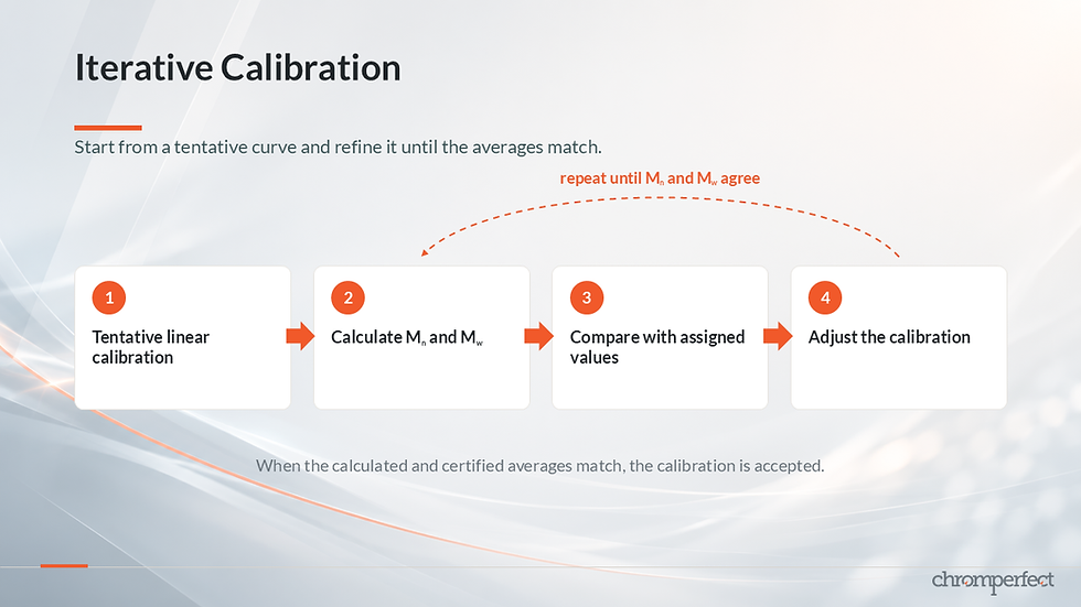
The method begins with a tentative linear relationship between log molecular weight and elution position. The broad-standard chromatogram is processed using this tentative curve, and calculated values of Mn and Mw are obtained.
The calibration is then adjusted iteratively until the calculated averages agree with the assigned values.
Once agreement is achieved, the positions corresponding to Mn and Mw become two calibration points.
A single broad standard produces two independent points, so it can support only a linear calibration.
Several broad standards can produce several pairs of points and may support a nonlinear calibration.

Column broadening and Hamilec calibration
The observed chromatographic profile is broader than the underlying molecular-weight distribution because of chromatographic dispersion.
For a broad standard, this additional spreading increases the apparent distance between the low- and high-molecular-weight portions of the chromatogram.
The Mn and Mw positions derived from the broadened profile are therefore farther apart than they would be without broadening.
As a result, the Hamilec calibration tends to rotate counterclockwise relative to the narrow-standard or “true” calibration curve.
The distorted calibration can partially compensate for similar broadening when samples are analysed. However, that compensation is reliable only when the sample resembles the standard in distribution shape and breadth.
If the sample distribution differs substantially from the standard, the compensation no longer matches and the calculated molecular-weight results may be inaccurate.

The Yau method
The Yau method is a modification of the Hamilec approach that attempts to correct the calibration for column broadening.
It introduces a value known as column sigma, σc.
Column sigma is the standard deviation, expressed in time or volume units, of the peak that a monodisperse sample would produce because of column and system broadening.
The Yau method uses the estimated column sigma to correct the calibration for the assumed contribution of broadening.
The corrected curve should lie closer to the underlying calibration relationship that would have been obtained using narrow standards.

The method assumes that column broadening can be represented by a single constant, σc.
In reality, broadening may vary with:
Elution position
Molecular size
Flow rate
Column condition
Other chromatographic factors
The Yau correction is therefore a model-based improvement rather than a perfect removal of chromatographic broadening.
An incorrect column-sigma estimate may under-correct or over-correct the calibration.
Integral, Hamilec and Yau methods compared
The three broad-standard methods differ principally in the information they require and in how they treat chromatographic broadening.
Integral method
Requires:
A cumulative molecular-weight-distribution table
Provides:
Several calibration points from one characterized broad standard
Limitation:
Accuracy depends on the quality of the distribution table and cumulative integration
Hamilec method
Requires:
Assigned Mn
Assigned Mw
Provides:
Two calibration points from one broad standard
Limitation:
The calibration is influenced by column broadening and by the distribution shape of the standard
Yau method
Requires:
Assigned Mn
Assigned Mw
Estimated column sigma, σc
Provides:
Two broad-standard points corrected using a broadening model
Limitation:
Accuracy depends on the validity of the constant-sigma assumption and the quality of the sigma estimate

Choosing an SEC calibration strategy
The most appropriate calibration method depends on the available standards and supporting physical information.
Use direct narrow-standard calibration when:
Suitable narrow standards are available
They are the same polymer type as the sample
They cover the required molecular-weight range
They are compatible with the selected solvent and temperature
Consider universal calibration when:
Standards are available for a chemically different polymer
Reliable Mark–Houwink constants or measured intrinsic viscosities are available
Information is available for both the standard and sample polymers
The separation is governed by size exclusion
Consider broad-standard calibration when:
Suitable narrow standards are unavailable
Universal calibration information is unavailable or unsuitable
A characterized broad standard is available
The broad-standard method then depends on the available characterization:
Molecular-weight-distribution table → Integral method
Mn and Mw → Hamilec method
Mn, Mw and σc → Yau method

What no SEC calibration method can overcome
No calibration model can compensate for unreliable standards or unsuitable chromatography.
A defensible SEC molecular-weight calibration requires:
Reliable assigned standard values
Chemically and physically stable standards
Appropriate detector response
Detector linearity
A correct SEC baseline
A correct processing range
Controlled flow rate
Controlled temperature
Separation governed primarily by size exclusion
A sophisticated calibration curve cannot recover information that is absent from the standards.
It also cannot correct:
Adsorption
Ionic interaction
Poor baseline selection
Detector saturation
Uncontrolled flow
Inappropriate processing limits
Unreliable physical constants

SEC calibration is a physical model
An SEC calibration curve should not be considered merely a mathematical line through a set of points.
It is a physical model connecting:
Elution behaviour
Effective molecular size
Molecular weight
Polymer chemistry
Intrinsic viscosity
Hydrodynamic volume
Chromatographic broadening
Every calculated molecular-weight value depends on the validity of that model and on the quality of the information used to build it.

Summary
SEC and GPC calibration convert chromatographic elution position into molecular-weight information.
For a polydisperse polymer, there is no single molecular weight. The material is described using averages including Mn, Mv, Mw, Mz and Mz+1, together with dispersity and the molecular-weight-distribution profile.
Direct narrow-standard calibration is normally the clearest approach when suitable standards of the same polymer are available.
Universal calibration provides a method for converting between chemically different polymers by using molecular-size-related information. The viscosity-based method uses the hydrodynamic-volume parameter [η]M and the Mark–Houwink relationship.
When suitable narrow standards are unavailable, characterized broad standards may be used through the Integral, Hamilec or Yau methods. Each approach requires different independent information and carries different assumptions about the standard distribution and chromatographic broadening.
The most appropriate SEC calibration method is therefore the one best supported by the available standards, physical constants, detector response and chromatographic conditions—not simply the method that is easiest to configure.
For the complete technical explanation, including the detailed development of each relationship and calibration method, watch the full SEC/GPC Theory Series Part 2 video at the top of this article.
Continue the SEC/GPC Theory Series
Part 1 — SEC Integration Theory
Part 1 explains the SEC baseline, detector noise, internal-standard correction, detector-response types and the calculations used to generate molecular-weight-distribution results.
Part 3 — Advanced SEC Theory
Part 3 continues with advanced interpretation of molecular-weight-distribution plots, axial correction, calculated-molecular-weight calibration plots and additional broad-standard information.
Frequently asked questions about SEC calibration
What is the difference between SEC and GPC?
SEC means size exclusion chromatography. GPC means gel permeation chromatography. GPC is commonly used for SEC analysis of polymers in organic solvents, while SEC is the broader term covering separation according to effective molecular size.
What does an SEC calibration curve show?
An SEC calibration curve relates elution time or elution volume to molecular weight, molecular size or hydrodynamic volume. It allows chromatographic detector response to be converted into a molecular-weight distribution.
Why is molecular weight plotted logarithmically in SEC?
SEC frequently covers several decades of molecular weight. A logarithmic scale gives each decade comparable graphical space and produces a more practical calibration relationship.
Why do large molecules elute first in size exclusion chromatography?
Large molecules enter fewer pores in the stationary phase and follow a shorter effective path through the column. Smaller molecules enter more pores and therefore elute later.
What is dispersity in polymer analysis?
Dispersity is the ratio Mw/MnM_w/M_nMw/Mn. It describes the breadth of a molecular-weight distribution. A monodisperse material has a value of one, while a polydisperse material has a value greater than one.
What is narrow-standard SEC calibration?
Narrow-standard calibration uses standards with sufficiently narrow molecular-weight distributions that their averages can be treated as approximately equal. Each standard peak top supplies one elution-position and molecular-weight calibration point.
What is universal calibration in GPC?
Universal calibration uses a molecular-size-related parameter rather than the molecular weight of one polymer. The most widely applicable method uses hydrodynamic volume, represented by the product of intrinsic viscosity and molecular weight, [η]M[\eta]M[η]M.
What is the Mark–Houwink relationship?
The Mark–Houwink relationship is:
[η] = κM^α
It connects intrinsic viscosity with molecular weight for a defined polymer, solvent and temperature combination.
What is a broad molecular-weight standard?
A broad standard contains a distribution of molecular weights rather than one narrow molecular-weight population. It cannot be represented by a single peak-top value and requires a distribution-aware calibration method.
What is the Integral method?
The Integral method uses a cumulative molecular-weight-distribution table for a broad standard. Cumulative chromatographic area percentages are matched to corresponding molecular weights to generate several calibration points.
What is the Hamilec method?
The Hamilec method uses the assigned Mn and Mw of a broad standard. A tentative linear calibration is adjusted iteratively until the calculated averages agree with the assigned values.
What is the Yau method?
The Yau method modifies Hamilec calibration by applying a correction based on the estimated column sigma, σc, to account for the assumed contribution of chromatographic broadening.
Can SEC calibration correct non-size-exclusion interactions?
No. Universal calibration and other mathematical methods cannot correct a fundamentally non-SEC separation caused by adsorption, ionic interaction or other non-size-exclusion retention mechanisms.
Which SEC calibration method should be used?
Use direct narrow-standard calibration when suitable same-polymer standards are available. Consider universal calibration when reliable viscosity or Mark–Houwink information exists for the standard and sample polymers. Use a broad-standard method when narrow standards and universal-calibration information are unavailable.

Comments