SEC/GPC Theory Series Part 3: Advanced SEC, Axial Correction and Molecular-Weight Distribution

This article forms Part 3 of the Chromperfect SEC/GPC Theory Series, created to provide a structured and detailed explanation of the principles behind size exclusion chromatography and gel permeation chromatography.
Part 1 of the series examines SEC integration theory, including baseline treatment, detector noise, detector-response types and the calculations used to convert an SEC chromatogram into molecular-weight information.
Part 2 covers SEC calibration theory, including molecular-weight averages, narrow-standard calibration, universal calibration, intrinsic viscosity, the Mark–Houwink relationship and broad-standard calibration methods.
Part 3 moves into advanced SEC theory, including the interpretation of molecular-weight-distribution plots, axial broadening, axial correction, calculated molecular-weight traces, local polydispersity, preparative fractionation and the creation of molecular-weight-distribution tables for broad standards.
This article accompanies our detailed video:
The video provides the complete technical presentation. This article summarizes the principal subjects and provides a structured written reference, but it should not be regarded as a replacement for the detailed visual explanations in the video.
What is advanced SEC theory?
Size exclusion chromatography, or SEC, separates dissolved molecules primarily according to their effective size in solution. In polymer analysis, SEC is also commonly known as gel permeation chromatography, or GPC.
Basic SEC analysis converts detector response versus elution time or elution volume into a molecular-weight distribution. Advanced SEC theory examines what happens after that conversion.
It addresses questions such as:
Why does an SEC molecular-weight-distribution plot contain several different traces?
Why do Mn, Mw, Mz and Mz+1 appear in particular positions?
Why does detector noise affect the number, weight and Z fractions differently?
How does chromatographic broadening change the apparent molecular-weight distribution?
What does axial correction attempt to calculate?
How can calculated Mn and Mw traces indicate local polydispersity?
How can cumulative weight fraction support preparative fractionation?
How can a broad polymer be characterized for use as an SEC standard?
These subjects are important because an SEC result is not simply one reported molecular-weight value. It is a description of a complete molecular population, interpreted through a chromatographic separation, a detector-response model and an SEC calibration relationship.
Understanding an SEC molecular-weight-distribution plot
A Chromperfect SEC molecular-weight-distribution plot can display a large amount of information.
Depending on the selected settings, as many as ten traces may be shown. These may include:
Number fraction
Weight fraction
Z fraction
Z-plus-one fraction
Viscosity fraction
Cumulative fraction traces
Molecular-weight-average markers
Other calculated distribution information
At first, the complete plot may appear complicated. However, fixed relationships exist among the traces, their positions and the molecular-weight markers.
Once these relationships are understood, the plot becomes much easier to interpret.

The basic idealized SEC example
The clearest way to understand the relationships is to begin with an idealized chromatogram.
Assume that:
The chromatogram contains one broad, symmetrical Gaussian peak.
There is no detector noise.
The detector is mass-sensitive.
The SEC calibration curve is linear.
Axial correction is not applied.
These assumptions remove the complications introduced by real detector noise, non-Gaussian distributions, calibration curvature and chromatographic broadening.
For the example used in the video, the midpoint of the SEC processing range corresponds to a molecular weight of 100,000 daltons.
The complete processing range spans slightly more than two decades of molecular weight. In logarithmic terms, one decade represents a tenfold molecular-weight range.
The original chromatographic peak is symmetrical, and its peak top corresponds to 100,000 daltons.
When the chromatogram is converted into a molecular-weight-distribution plot, the horizontal axis changes from elution time or elution volume to molecular weight.
The chromatographic response remains Gaussian, but the meaning of the axis has changed.

Why the weight-fraction trace resembles the chromatogram
For a mass-sensitive detector, the measured detector response is proportional to the mass of material eluting.
The weight-fraction trace therefore reproduces the shape of the original chromatogram. The principal difference is that the horizontal axis now represents molecular weight rather than elution time.
This relationship depends on the detector-response type.
It is not correct to assume that the original chromatogram always represents weight fraction.
The trace corresponding directly to the measured chromatogram depends upon whether the detector response is treated as:
Mass-sensitive
Mole-sensitive
Z-sensitive
With a mass-sensitive detector, the measured response corresponds to weight fraction.
With a mole-sensitive detector, the number-fraction trace corresponds more directly to the measured chromatogram.
With an idealized Z-sensitive detector, such as the theoretical response of a low-angle light-scattering detector, the Z-fraction trace becomes the reference trace.
Correct declaration of detector type in the SEC Calibration file is therefore required for both correct molecular-weight calculations and correct interpretation of the molecular-weight-distribution plot.

Cumulative weight fraction
The cumulative weight-fraction trace is the integral of the weight-fraction trace.
It is normalized so that it begins at zero and ends at one, or from zero to 100 percent when expressed as a percentage.
At any molecular weight, the cumulative trace indicates how much of the sample has already been accounted for on one side of that position.
For a symmetrical Gaussian distribution, the cumulative trace reaches 0.5 at the molecular-weight position directly beneath the peak top.
The cumulative weight-fraction trace becomes particularly useful later when selecting preparative fraction boundaries or creating a broad-standard molecular-weight-distribution table.

Number-average and weight-average molecular weight
The molecular-weight-distribution plot may display markers for the calculated molecular-weight averages.
The most familiar are:
Number-average molecular weight, Mn
Weight-average molecular weight, Mw
For a conventional SEC molecular-weight-distribution plot:
High molecular weight appears on the left.
Low molecular weight appears on the right.
Mn lies toward the low-molecular-weight side of the peak top.
This occurs because the low-molecular-weight region contains a greater number of individual polymer molecules.
Mw lies toward the high-molecular-weight side.
This occurs because larger molecules make a stronger contribution to the weight average.
For a polydisperse polymer, the normal relationship is:
Mn < Mw
The distance between the Mn and Mw markers is related to the breadth of the molecular-weight distribution.
A narrow distribution produces Mn and Mw markers that are close together.
A broader distribution produces markers that are farther apart.
This relationship is commonly expressed using dispersity:
Đ = Mw / Mn
For an ideal monodisperse material:
Mw = Mn
and therefore:
Đ = 1
Marker spacing must also be interpreted in the context of the SEC calibration-curve slope.
A steep calibration curve converts a small difference in elution time into a comparatively large molecular-weight difference. The same chromatographic peak width may therefore produce greater spacing between the molecular-weight averages.

Number, weight, Z and Z-plus-one fraction traces
The principal differential molecular-weight-distribution traces are:
Number fraction
Weight fraction
Z fraction
Z-plus-one fraction
For the idealized Gaussian chromatogram and linear SEC calibration curve, the four traces have several regular properties:
They remain Gaussian.
They have the same height.
They have the same width.
They are displaced along the molecular-weight axis.
The spacing between adjacent traces is equal.
From low molecular weight toward high molecular weight, the order is:
Number fraction → Weight fraction → Z fraction → Z-plus-one fraction
On a conventional plot with high molecular weight on the left, the visual order from left to right is therefore:
Z-plus-one → Z → Weight → Number
Each higher-order trace applies progressively greater emphasis to the high-molecular-weight region.

Why the markers appear at trace intersections
The molecular-weight-average markers occur where adjacent fraction traces intersect.
The key relationships are:
Mn = intersection of number fraction and weight fraction
Mw = intersection of weight fraction and Z fraction
Mz = intersection of Z fraction and Z-plus-one fraction
Mz+1 does not have an equivalent final intersection because no Z-plus-two fraction is displayed.
These relationships provide a useful visual check when reading an SEC molecular-weight-distribution plot.
Even when a real distribution is irregular or multimodal, the order of the fraction traces and the relationship between the markers and their intersections should generally remain recognizable.

Viscosity fraction and viscosity-average molecular weight
The viscosity fraction and viscosity-average molecular weight, Mv, introduce another trace and marker.
Their positions depend upon the Mark–Houwink exponent, alpha.
When alpha = 0:
Viscosity fraction = Weight fraction
Chromperfect reports:
Mv = Mw
When 0 < alpha < 1:
The viscosity fraction lies between the weight and Z fractions.
When alpha = 1:
Viscosity fraction = Z fraction
When 1 < alpha < 2:
The viscosity fraction lies between the Z and Z-plus-one fractions.
When alpha = 2:
Viscosity fraction = Z-plus-one fraction
The Mv marker occurs where the weight-fraction and viscosity-fraction traces intersect.
As alpha increases, the viscosity-fraction trace and Mv marker move toward higher molecular weight.
Near alpha = 0, Mv lies approximately halfway between the positions of Mn and Mw.
At alpha = 2, Mv lies approximately halfway between the positions of Mw and Mz.
This does not mean that Mv is the arithmetic average of those molecular-weight values. It describes its approximate graphical position on the molecular-weight axis.
Mv therefore cannot be interpreted independently of the polymer, solvent, temperature and applicable Mark–Houwink relationship.

Real SEC chromatograms
The idealized Gaussian example provides a clear framework, but real SEC chromatograms are more complicated.
A real sample may contain:
Several overlapping molecular-weight regions
Asymmetrical distributions
Detector noise
Weak distribution tails
Irregular peak shapes
Calibration curvature
Consider a chromatogram containing three broad, overlapping Gaussian peaks with a small amount of detector noise.
When converted into number, weight, Z and Z-plus-one traces, the profiles no longer have identical shapes, heights or widths.
The weight-fraction trace continues to reproduce the original chromatogram when the detector is mass-sensitive.
The number fraction emphasizes the later-eluting, low-molecular-weight region.
The Z fraction emphasizes earlier-eluting, high-molecular-weight material.
The Z-plus-one fraction emphasizes the extreme high-molecular-weight region even more strongly.

Molecular-weight markers in a complex distribution
In a broad or multimodal distribution, the molecular-weight-average markers are generally farther apart than in a narrow Gaussian example.
The markers are no longer equally spaced because the distribution is not represented by one simple Gaussian population.
Nevertheless, the fundamental order remains:
Mn < Mw < Mz < Mz+1
When displayed on a conventional molecular-weight axis, Mn lies toward the low-molecular-weight side, while the higher-order averages move progressively toward the high-molecular-weight side.
The intersections between corresponding traces also remain meaningful.

Why noise affects each trace differently
Detector noise appears in every calculated distribution trace, but each trace weights that noise differently.
For a mass-sensitive detector:
The weight-fraction trace reproduces detector noise directly.
The number-fraction trace increases the influence of late-eluting, low-molecular-weight noise.
The Z and Z-plus-one traces increase the influence of early-eluting, high-molecular-weight noise.
This effect is important because a small fluctuation in the high-molecular-weight region can have a disproportionate influence upon Mz and Mz+1.
Noise should therefore be considered whenever:
A distribution trace appears irregular.
Molecular-weight markers move unexpectedly.
Higher-order averages appear unstable.
Weak distribution tails exert an unusually large influence.

What is axial broadening in SEC?
Ideal SEC would introduce the sample in an infinitesimally small volume and separate molecules without adding any additional spreading.
Real chromatography cannot fully attain this condition.
Broadening can be introduced by:
Finite injection volume
Connections and tubing
Detector-cell volume
Diffusion
Mass-transfer effects
Other extra-column volumes
Within the column, material spreads longitudinally along the direction of flow. This is commonly described as axial broadening.
The observed molecular-weight distribution is therefore broader than the true molecular-weight distribution entering the chromatographic system.

Observed width, true width and column sigma
For Gaussian distributions, the relationship between the observed distribution, the true sample distribution and chromatographic broadening can be described using variances.
sigma-observed² = sigma-sample² + sigma-column²
Where:
sigma-observed is the standard deviation of the observed chromatographic distribution.
sigma-sample is the genuine standard deviation of the sample distribution.
sigma-column is the broadening introduced by the complete chromatographic system.
In Chromperfect, column sigma is expressed in time or volume units.
A perfectly monodisperse standard has no genuine molecular-weight-distribution width.
However, it still produces a chromatographic peak with a finite observed width.
Under the axial-broadening model, that observed width represents broadening introduced by the chromatographic system.
A broad polymer has its own genuine distribution width. Column broadening is superimposed upon it, causing the observed chromatogram to exaggerate the breadth of the original molecular-weight distribution.

Consequences of axial broadening
Axial broadening affects several calculated properties.
It can:
Increase apparent dispersity
Move Mn toward lower molecular weight
Move Mw toward higher molecular weight
Affect Mz and Mz+1 even more strongly
Mix material between neighboring apparent fractions
Reduce the apparent purity of preparative fractions
Broadening increases the spacing between molecular-weight-average markers because it makes the observed distribution appear wider.
Higher-order averages are particularly sensitive because they give greater mathematical emphasis to the extreme high-molecular-weight region.

Neighboring fractions become mixed
A fraction observed at one elution time does not contain only molecules whose ideal elution position corresponds exactly to that time.
Instead, it contains contributions from neighboring positions on both sides.
This contamination is especially important in:
Preparative SEC
Selection of collection windows
Broad-standard calibration
Local polydispersity calculations
The ordinary SEC calculation assigns one molecular weight to each chromatographic data point using the calibration curve.
Axial correction treats each observed point as a weighted mixture of contributions from neighboring ideal positions.

How the axial-correction model works
The contribution from each neighboring position depends upon two factors:
The amount of material present at that position
The distance between that position and the observed point
The distance weighting is represented by a Gaussian distribution whose standard deviation is equal to column sigma.
Nearby positions contribute more strongly than distant positions.
The weighted neighboring detector responses and their ordinary molecular weights are then used to calculate corrected molecular-weight averages for each observed chromatographic point.
Axial correction does not reconstruct an exact original chromatogram.
It applies a mathematical model intended to estimate the molecular-weight distribution that might have been observed with less chromatographic broadening.

Assumptions and limitations of axial correction
The axial-correction model depends upon several assumptions.
It assumes that:
Broadening is Gaussian.
A single column-sigma value adequately represents the complete chromatographic system.
The selected sigma value is physically realistic.
The baseline and detector response are reliable.
Genuine distribution tails can be distinguished from noise.
I
n reality, chromatographic broadening may vary with:
Molecular size
Flow rate
Diffusion coefficient
Column condition
Injection volume
Extra-column volume
Position within the separation range
A single column-sigma value is therefore an approximation.
If column sigma is too small, the correction has little practical effect and the calculated molecular-weight traces remain close to the ordinary calibration curve.
If column sigma is too large, the correction may become physically unrealistic.
An excessive value may produce a positive molecular-weight slope. In conventional SEC, molecular weight must decrease as elution time increases.

Noise, smoothing and the SEC noise threshold
Axial correction is sensitive to detector noise because it uses neighboring detector responses and high powers of molecular weight.
Noise is especially influential near the beginning and end of a chromatographic peak, where genuine analyte response is weak.
Two settings can help:
Chromatographic smoothing
The SEC noise threshold
A suitable noise threshold can prevent low-response regions from being included in corrected calculations.
Smoothing may reduce jitter in the calculated traces.
However, either treatment can become excessive.
A threshold that is too high excludes genuine molecular-weight-distribution tails.
Excessive smoothing changes the chromatographic profile and may conceal real distribution features.
The analyst must therefore balance noise rejection against preservation of genuine low-level material.

Calculated molecular-weight calibration plots
The SEC Calibration File Editor displays calibration curves stored in an SEC Calibration file.
However, the editor is not associated with a Raw Data file or Bound file. It therefore cannot display corrected values calculated from an actual chromatogram.
Chromatogram-dependent calculated molecular-weight traces can be displayed in:
Chromperfect Analysis
Formatted reports
When axial correction is enabled, a calculated-MW plot may contain:
The ordinary calibration curve
Calculated sample Mn
Calculated sample Mw
Calculated sample Mz
Other corrected molecular-weight averages

Why calculated traces contain gaps and jitter
Not every acquired chromatographic point is included in a calculated molecular-weight trace.
A point must normally be:
Inside the SEC processing range
Above the SEC noise threshold
Points below the threshold are excluded. The resulting calculated trace may therefore contain gaps or discontinuities.
The ordinary calibration curve remains smooth because it is a stored mathematical relationship.
The corrected molecular-weight traces are commonly more irregular because they depend upon:
Actual detector response
Neighboring chromatographic points
Axial-correction settings
Baseline noise
Processing limits
Smoothing and threshold settings
Irregularity is usually most pronounced near the distribution ends.

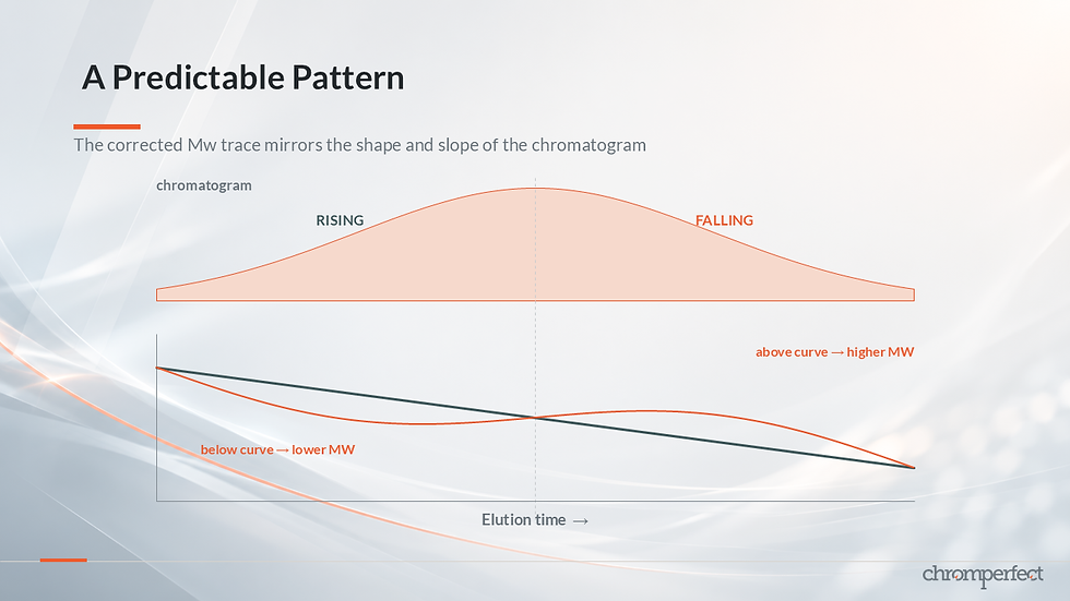
Why corrected Mw follows the chromatogram
The corrected sample Mw trace typically moves above and below the ordinary calibration curve.
This behavior reflects the slope of the chromatographic response.
Where the chromatogram is rising:
More neighboring contribution arrives from later-eluting material.
Later-eluting material has lower molecular weight.
Corrected Mw shifts downward toward lower molecular weight.
Where the chromatogram is falling:
More neighboring contribution arrives from earlier-eluting material.
Earlier-eluting material has higher molecular weight.
Corrected Mw shifts upward toward higher molecular weight.
This is not random movement. It is the expected result of the neighboring-point contamination model.
Local polydispersity
Calculated local Mn and Mw traces provide information about the breadth of the molecular population at individual chromatographic positions.
Where local Mn and Mw are nearly coincident, the local fraction is relatively narrow.
Where the traces separate, local polydispersity is greater.
Local polydispersity = local Mw / local Mn
At the top of a chromatographic peak, there may be comparatively little contamination from either side. The local fraction may therefore appear relatively narrow.
In a valley between two overlapping distributions, material contributes from both sides. The local fraction may contain molecules from two substantially different molecular-weight regions.
Its calculated polydispersity is therefore higher.

Selecting preparative fractions using local polydispersity
Local polydispersity information can help identify where preparative collection cuts should be placed.
A cut through a region where local Mn and Mw are close together may produce a relatively narrow fraction.
A cut through a region of high local polydispersity may collect a mixture of neighboring molecular-weight populations.
The best collection region is therefore not determined only by detector-response height.
The local breadth and purity of the fraction should also be considered.

Validating the column-sigma value
Calculated molecular-weight traces can help determine whether the selected column-sigma value is plausible.
If sigma is too small:
The calculated traces remain close to the ordinary calibration curve.
The correction has little effect.
If sigma is too large:
The calculated traces may become physically unrealistic.
A positive molecular-weight slope may appear.
A plausible correction should remain consistent with conventional SEC behavior, in which molecular weight generally decreases with increasing elution time or volume.
The analyst should compare:
The chromatogram
The ordinary calibration curve
The calculated molecular-weight traces

Noise and numerical resolution
Axial-correction calculations are sensitive not only to detector noise but also to numerical roundoff.
The calculation may involve:
Very large powers of molecular weight
Small differences among weighted sums
Finite digital precision
In normal applications, these effects are usually negligible.
They become visible in deliberately extreme examples.
Suppose that:
sigma-column² = sigma-observed²
From:
sigma-observed² = sigma-sample² + sigma-column²
the model infers:
sigma-sample² = 0
The calculated true sample is therefore treated as perfectly monodisperse.
Ideally:
Mn = Mw = Mz = Mz+1
All molecular-weight-average traces should become horizontal and overlap.
In practice, detector noise and numerical precision may produce small discrepancies.
When highly magnified, these differences can appear more important than they are.

Molecular-weight resolution per data point
The sampling interval and calibration-curve slope place a fundamental limit on molecular-weight resolution.
Change in log molecular weight per point = calibration-curve slope × sampling interval
Or:
Delta log(M) = calibration slope × sampling interval
If consecutive acquired points differ by approximately 0.3 percent in molecular weight, calculated differences much smaller than 0.3 percent cannot be interpreted reliably.
A higher sampling rate reduces the time interval between points and may improve resolution to a limited degree.
However, oversampling cannot recover information already lost through:
Chromatographic broadening
Detector noise
Inadequate separation
Higher-order averages such as Mz and Mz+1 are also more susceptible to roundoff because they use higher powers of molecular weight.
For an apparently monodisperse material, Mn and Mw generally provide the more stable assessment.
A dispersity result such as:
Đ = 1.0004
may represent monodispersity within the practical resolution of the acquisition system rather than a physically meaningful difference from 1.

Fractionating a broad molecular-weight-distribution polymer
Narrow molecular-weight standards can be produced by fractionating a broad polymer.
Preparative SEC is frequently used for this purpose.
A typical process includes:
Analyze a small quantity of the broad polymer.
Identify suitable collection regions.
Separate a larger quantity under preparative conditions.
Collect the selected fractions.
Concentrate each collected fraction.
Chromatograph each fraction again.
Retain the central portion.
Discard the leading and trailing portions.
Determine Mn and Mw independently.
Repeat the process if the fraction remains too broad.
Repeated fractionation moves Mn and Mw closer together.
Eventually, the fraction may become effectively monodisperse within the precision of the physical measurement.

The yield versus purity trade-off
Complete fractionation is rarely practical.
If only the middle half of a distribution is retained at each stage, the available material decreases rapidly:
100 percent → 50 percent → 25 percent → 12.5 percent
This is a conceptual example, but it demonstrates the practical cost of repeated purification.
The objective is not always perfect monodispersity.
A useful fractionation strategy balances:
Distribution width
Material yield
Intended use of the standard

Selecting approximately equal-mass fraction boundaries
Chromperfect can provide information to help select preparative fraction boundaries.
Consider a broad polymer with three overlapping molecular-weight regions that must be divided into seven fractions of approximately equal mass.
For a suitable mass-sensitive detector, detector-response area is assumed to be proportional to mass.
The cumulative weight-fraction trace shows how much sample mass has been accounted for across the molecular-weight distribution.
Preliminary fraction boundaries can be positioned at:
1/72/73/74/75/76/7
of cumulative mass.
These positions create seven fractions of approximately equal mass, although their molecular-weight widths may differ.

What Chromperfect can report for each fraction
A formatted report can calculate the following for each proposed slice:
High molecular-weight limit
Low molecular-weight limit
Mn
Mw
Mw divided by Mn
Weight fraction
Cumulative fraction
Initial boundaries will not usually produce perfectly equal fractions.
The slice limits can be adjusted iteratively until the weight fractions become acceptably uniform.
Once the fractions have similar mass, their Mn, Mw and dispersity values can be examined to determine whether additional fractionation is required.
The molecular-weight-distribution plot therefore supports both:
Equal-mass division
Assessment of expected fraction width and purity

Creating an MWD table for a broad standard
Suitable narrow molecular-weight standards are not always available.
A broad polymer may still be used as an SEC standard if its molecular-weight distribution is known independently.
An MWD table relates cumulative sample fraction to molecular weight.
For example, it may contain the molecular weight corresponding to:
10 percent cumulative mass
20 percent cumulative mass
30 percent cumulative mass
Continuing through 90 percent cumulative mass
The central portion of the distribution is normally more reliable than the extreme tails.

Generating a candidate broad-standard table
A candidate broad standard can be processed using an existing SEC calibration believed to be reliable.
A formatted report can calculate cumulative molecular-weight values at selected cumulative fractions.
Possible report series include:
Cumulative Mn
Cumulative Mw
Cumulative Mz
The software’s ability to calculate these values does not establish that any particular series is physically appropriate.
The analyst must select the series supported by independent characterization.
The reliability of the resulting table depends upon:
The source calibration
Detector-response type
Baseline quality
Processing range
Noise treatment
Standard stability
Distribution breadth
Independent traceability

Designing a defensible MWD table
A useful broad-standard table should contain several well-spaced entries across the central part of the distribution.
Values close to zero or 100 percent cumulative fraction are vulnerable to:
Detector noise
Baseline uncertainty
Small integration errors
Large molecular-weight errors caused by weak response
Well-spaced intermediate cumulative fractions generally provide more defensible calibration information.
The resulting cumulative percentages and molecular weights can be entered into a new SEC Calibration file for use with the broad-standard integral method.

Why a derived calibration cannot validate itself
An MWD table derived from SEC is not automatically an independent primary measurement.
If the table is created using an existing SEC calibration, it inherits the assumptions and errors of that calibration.
The resulting table may be useful for:
Transferring a calibration
Reproducing a calibration
Working under similar chromatographic conditions
However, it cannot independently validate itself.
Using an existing SEC calibration to create an MWD table and then using that table to confirm the original calibration creates circular reasoning.

Traceability and independent characterization
Ideally, a broad standard should be characterized using:
Independent physical measurements
Separately characterized fractions
Molecular weights established outside the SEC calibration being created
When an MWD table is derived chromatographically, the following should be documented:
Source calibration
Assumptions
Traceability
Detector-response model
Processing conditions
Known limitations
This documentation makes clear what the derived table can and cannot establish.

Advanced SEC theory in Chromperfect
Advanced SEC analysis moves beyond a single reported average molecular weight.
It examines:
The complete molecular-weight distribution
Number, weight, Z and viscosity-related fraction traces
Molecular-weight-average marker relationships
Detector-response dependence
Chromatographic broadening
Axial-correction assumptions
Corrected molecular-weight traces
Local polydispersity
Preparative fraction purity
Molecular-weight resolution
Broad-standard characterization
These calculations can provide valuable insight, but they must always be interpreted within the practical limits of the chromatography, detector response, calibration method, data-acquisition rate and numerical model.
Axial correction cannot recreate information that was never resolved by the chromatographic system.
A calculated molecular-weight difference is not necessarily physically meaningful simply because it can be displayed with several decimal places.
Likewise, an MWD table is only as reliable as the independent measurements, source calibration and experimental controls supporting it.
Watch the complete SEC/GPC Theory Series
The Chromperfect SEC/GPC Theory Series provides a structured explanation of SEC integration, calibration and advanced molecular-weight-distribution analysis.
Part 1 — SEC Integration Theory -
Covers SEC baseline treatment, detector noise, internal-standard correction, detector-response types and molecular-weight calculations.
Part 2 — SEC Calibration Theory
Explains molecular-weight averages, narrow-standard calibration, universal calibration, hydrodynamic volume, intrinsic viscosity, Mark–Houwink relationships and broad-standard calibration methods.
Part 3 — Advanced SEC Theory
Examines molecular-weight-distribution plots, axial broadening, axial correction, calculated molecular-weight traces, local polydispersity, preparative fractionation and broad-standard MWD tables.

Learn more about Chromperfect
Chromperfect chromatography software supports SEC/GPC analysis, molecular-weight-distribution calculations, calibration workflows, formatted reporting and advanced polymer-characterization applications.
For chromatography software, technical resources, training articles and product information, visit:


Comments