SEC/GPC Theory Series Part 1: SEC Integration, Baselines and Molecular-Weight Calculations

This article forms Part 1 of the Chromperfect SEC/GPC Theory Series, created to provide a structured and detailed explanation of the principles behind size exclusion chromatography and gel permeation chromatography.
Part 1 (This article) examines SEC integration theory, including the dedicated SEC baseline, detector noise, internal-standard flow correction, detector-response types and the calculations used to convert an SEC chromatogram into molecular-weight information
.
Part 2 covers SEC calibration theory, including molecular-weight averages, narrow-standard calibration, universal calibration, intrinsic viscosity, the Mark–Houwink relationship and broad-standard calibration methods.
Part 3 moves into advanced SEC theory, including molecular-weight-distribution plots, axial broadening, axial correction, calculated molecular-weight traces, local polydispersity and preparative fractionation.
This article accompanies our detailed video:
The video provides the complete technical presentation. This article summarizes the principal subjects and provides a structured written reference, but it should not be regarded as a replacement for the detailed visual explanations in the video.
Although Chromperfect software is referenced throughout the presentation, the underlying scientific principles apply broadly to SEC/GPC analysis and to other chromatography data systems.
What is SEC integration theory?
Size exclusion chromatography, commonly abbreviated as SEC and also known as gel permeation chromatography or GPC, differs from conventional chromatography in an important way.
In ordinary chromatography, integration normally involves:
Detecting separate chromatographic peaks
Establishing a baseline beneath each peak or peak cluster
Identifying the corresponding components
Calculating peak area, height or concentration
An SEC chromatogram may instead represent a continuous distribution of polymer molecules having different sizes and molecular weights.
The objective is therefore not simply to measure a collection of independent peaks. SEC integration determines how detector response is distributed across the molecular-weight range and uses that information to calculate molecular-weight averages, intrinsic viscosity and molecular-weight fractions.
The complete calculation can be summarized as:
Raw Data → SEC Baseline → Flow Correction → SEC Calibration Curve → Molecular-Weight Calculations → Results

How the SEC baseline differs from ordinary peak baselines
SEC integration uses one dedicated baseline for the complete SEC processing range.
This baseline is separate from the individual peak baselines that may be produced during ordinary chromatographic integration.
Conventional integration may create several different baselines beneath individual peaks or peak clusters. SEC integration instead requires one common reference against which detector response across the complete molecular-weight distribution can be measured.
The SEC baseline may be:
Horizontal
Sloping
A horizontal baseline is established using one baseline anchor.
A sloping baseline is established using two anchors, with a straight line drawn between their calculated positions.
How SEC baseline anchors are calculated
The elution times of the baseline anchors are defined in the SEC Calibration file.
At each anchor time, Chromperfect locates the five nearest points in the Raw Data file and calculates their average detector response.
That average establishes the baseline height at the anchor.
The process is:
Anchor time → Five nearest Raw Data points → Average detector response → Baseline position
With one anchor, the resulting SEC baseline is horizontal.
With two anchors, Chromperfect draws a straight line between the two averaged anchor positions. This allows the SEC baseline to follow gradual detector drift across the analysis.

Choosing suitable SEC baseline-anchor positions
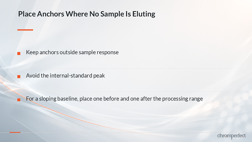
Although baseline anchors can technically be placed anywhere in the chromatogram, they should be positioned where no sample material is eluting.
They should also be kept away from the SEC internal-standard peak when an internal standard is being used.
For a horizontal baseline, a single anchor may be placed at time zero when that position provides a representative baseline response.
For a sloping baseline, one anchor is normally positioned before the SEC processing range and the second after it.
The purpose is to measure detector response on either side of the molecular-weight distribution without allowing sample response to influence the baseline position.
Poorly chosen baseline anchors can distort the apparent distribution and therefore affect every molecular-weight result calculated from it.
Managing detector noise in SEC integration
Even when no analyte is eluting, a detector does not normally produce a perfectly flat signal.
Baseline variation may result from:
Electronic noise
Pump effects
Temperature variation
Short-term detector instability
Other instrumental influences
Small fluctuations above and below the SEC baseline may appear insignificant when viewed as detector response. However, their influence can become much greater after each point has been assigned a molecular weight.
For this reason, baseline treatment is especially important in SEC/GPC analysis.
Clamp and flip treatment of negative response
Detector excursions below the SEC baseline require specific treatment.
Chromperfect can apply either clamp or flip behavior to negative SEC response.
Clamp
Clamping treats negative detector response as zero relative to the SEC baseline.
The negative excursion does not contribute to the molecular-weight calculation.
Flip
Flipping converts the negative excursion into an equivalent positive response above the baseline.
The magnitude of the signal is retained, but its direction is reversed.
The correct choice depends on the physical meaning of the detector response.
Flipping is appropriate only when a negative signal genuinely represents analyte and its magnitude remains analytically meaningful.
Clamping is appropriate when the negative excursion represents noise, baseline instability or another response that should not contribute to the molecular-weight distribution.

Why early-eluting detector noise is particularly important
In conventional SEC, earlier elution normally corresponds to larger molecular size and therefore higher calculated molecular weight.
A small amount of apparent detector response near the beginning of the SEC processing range may consequently be assigned an extremely high molecular weight.
Although the detector response itself may be very small, the molecular-weight weighting used in higher-order calculations can give that point a disproportionate influence.
This is particularly important for:
Z-average molecular weight, Mz
Z-plus-one average molecular weight, Mz+1
High-molecular-weight fractions
Axially corrected calculations
A small early-eluting fluctuation may have little influence on Mn but a much larger influence on Mz or Mz+1.

Using the SEC noise threshold
The SEC Calibration file provides a noise threshold to prevent low-level detector fluctuations from contributing to the calculation.
Detector response below the selected threshold is ignored.
The threshold must be selected carefully:
It should be high enough to exclude detector noise.
It should not be so high that genuine low-level polymer response is removed.
An excessive noise threshold may truncate genuine molecular-weight-distribution tails.
A threshold that is too low may allow noise to influence molecular-weight averages and fractions.
This setting is particularly important when an SEC calibration is created from a broad molecular-weight standard whose distribution table includes cumulative values of zero or 100 percent. At these extremes, very small amounts of detector noise can interfere with the relationship between chromatographic response and the stated molecular-weight distribution.
Smoothing SEC chromatograms
Smoothing provides another method for reducing the influence of short-term detector noise.
Appropriate smoothing can:
Improve SEC baseline placement
Reduce the need for an excessively high noise threshold
Improve measurement of narrow-standard elution times
Reduce short-term variation in calculated SEC traces
However, smoothing must be used cautiously.
Every SEC column broadens the sample distribution to some extent. The smoothing time constant must remain substantially smaller than the peak broadening produced by the chromatographic system.
If smoothing is excessive, it can alter the apparent molecular-weight distribution and introduce additional error.
The objective is to reduce short-term detector noise without materially changing the chromatographic profile generated by the SEC separation.

The purpose of an SEC internal standard
SEC integration can use an internal standard, but its purpose differs from that of a conventional quantitative internal standard.
In quantitative chromatography, an internal standard may be used to correct for variations in:
Sample preparation
Injection volume
Detector response
Quantitative recovery
The SEC internal standard described here does not perform this function.
It is used only as an elution-time reference for correcting between-run variation in average flow rate.

Elution volume and flow-rate stability
Strictly speaking, SEC separates molecules according to elution volume rather than elution time.
Elution volume can be expressed as:
Ve = F × te
where:
Ve is elution volume
F is mobile-phase flow rate
te is elution time
Modern chromatography pumps normally provide sufficient short-term stability for elution time to be used as a practical substitute for elution volume.
However, this substitution depends on flow rate remaining consistent.
SEC calibration commonly relates elution time or volume to the logarithm of molecular weight. A relatively small shift in average flow rate can therefore cause a much larger error in calculated molecular weight.

What SEC flow correction can and cannot do
The internal standard can correct a difference in average flow rate between:
The run used to establish the SEC calibration
A later sample analysis
A broad-standard calibration analysis
It cannot correct a flow rate that changes during an individual chromatographic run.
The correction assumes that the complete time axis has been displaced by a consistent change in average flow.
If flow changes progressively or irregularly during the run, one correction factor cannot restore the correct relationship across the complete chromatogram.
Selecting an SEC internal standard
The SEC internal standard should have a sufficiently low molecular weight to be fully included by the column packing.
A fully included molecule can enter essentially all accessible pore volume.
Its elution volume therefore includes both:
The excluded volume of the chromatographic system
The included pore volume accessible to the molecule
Because the internal standard elutes near the end of the useful separation range, its position reflects average flow over most of the chromatographic run.
The expected internal-standard elution time and the width of its search window are defined in the SEC Calibration file.
The internal-standard peak must still be detected by ordinary chromatographic peak integration. However, it does not need to be identified as a component in an ordinary Calibration file, and an ordinary Calibration file is not required for the SEC flow correction.
How internal-standard time correction is applied
Chromperfect compares:
The observed internal-standard elution time
The expected internal-standard elution time
The correction is based on the ratio between these two values.
The sequence is:
Observed internal-standard time→ Expected-to-observed time ratio→ Corrected chromatographic time axis→ SEC calibration relationship→ Molecular weight or hydrodynamic volume
This order is important.
Chromperfect first adjusts the chromatographic time axis to compensate for the estimated difference in average flow rate. It then applies the SEC calibration relationship to the corrected times.
The internal-standard correction is applied to:
SEC sample analyses
Broad-standard SEC calibration
It is not applied during narrow-standard SEC calibration because the observed elution time of each narrow standard is itself used to establish the calibration curve.

Why detector linearity matters in SEC/GPC
The SEC integration calculation assumes that detector response remains proportional to the amount of material passing through the detector.
The full SEC chromatogram must therefore remain within the detector’s usable linear-response range.
The SEC calibration curve does not correct detector nonlinearity.
An SEC calibration curve relates chromatographic position to molecular weight or hydrodynamic volume. It does not repair an incorrect relationship between analyte quantity and detector response.
If the detector becomes saturated, or its response is otherwise nonlinear, the apparent shape of the molecular-weight distribution becomes distorted.
This can affect:
Mn
Mw
Mz
Mz+1
Intrinsic viscosity
Molecular-weight fractions
Distribution breadth
Detector linearity should therefore be established rather than assumed.
A practical approach is:
Prepare dilutions → Perform multilevel calibration → Compare detector response → Establish the maximum linear response
Only detector responses within the demonstrated linear range should be used for reliable molecular-weight calculations.

Between-run and within-run sensitivity changes
SEC calculations are normally based on relative detector response.
A consistent proportional change in detector sensitivity between runs does not necessarily alter the calculated distribution. If every point in the chromatogram changes by the same proportion, the relative response profile remains unchanged.
A sensitivity change during a single run is different.
If detector sensitivity changes while the distribution is eluting, different molecular-weight regions are affected by different amounts. The calculated distribution and its molecular-weight averages may then become incorrect.
Adequate detector warm-up and stable operating conditions are therefore important.
SEC detector-response types
The physical meaning of detector response is critical to the SEC calculation.
Chromperfect supports several response models, including:
Mass-sensitive response
Mole-sensitive response
Low-angle light-scattering response
Viscosity-sensitive response
The same polymer distribution produces different mathematical response profiles depending on what the detector measures.

Mass-sensitive detector response
For a mass-sensitive detector, response is proportional to the mass of solute in the detector cell.
Equal mass produces the same idealized response regardless of how that mass is divided among individual molecules.
For example, one gram of material produces the same idealized response whether it consists of:
Many small molecules
Fewer large molecules
This assumes that all other detector-response factors remain equal.
With a mass-sensitive detector:
Total chromatographic area is proportional to total analyte mass.
Response at each elution position is proportional to the mass passing through the detector at that time.
Refractive-index detectors are commonly treated as mass-sensitive when the relationship between concentration and refractive-index response is suitable.
Mole-sensitive detector response
A mole-sensitive detector responds according to the number of molecules rather than their combined mass.
One example is a detector responding to a labeled polymer end group where every molecule carries one identical label.
A small molecule and a large molecule may each contain one labeled end group and therefore contribute one response unit.
With a mole-sensitive detector:
Total chromatographic area is proportional to the total number of molecules.
Response at each elution position is proportional to the number of molecules passing through the detector.
Low-angle light-scattering response
For an idealized low-angle light-scattering detector, response is proportional to the number of molecules multiplied by the square of molecular weight:
Response ∝ Number of molecules × M²
This response applies much greater weighting to large molecules.
It is commonly described as a Z-sensitive response because of its relationship to the higher-order molecular-weight calculations.
Viscosity-sensitive detector response
A viscosity-sensitive detector responds to the viscosity of the eluting polymer solution.
This response is related to the hydrodynamic volume of the polymer molecules in the detector cell.
With a viscosity-sensitive detector:
Total area is proportional to the total hydrodynamic volume of the analyte.
Response at each elution position is proportional to the hydrodynamic volume passing through the detector.
Chromperfect converts the declared detector response into consistent molar units before applying the common molecular-weight equations.
Selecting the wrong response type changes the mathematical interpretation of every chromatographic point and therefore changes the calculated molecular-weight distribution.

Limitations of refractive-index detection
Even when detector response appears linear, additional physical limitations may affect quantitative SEC measurement.
For some analytes, refractive index changes with molecular weight.
Detector sensitivity per unit mass may therefore vary across the polymer distribution.
A more serious situation occurs when the refractive index of the analyte crosses that of the solvent.
At the crossing point:
The refractive-index difference becomes zero.
Detector response may disappear even though analyte remains present.
The signal may reverse direction after the crossing point.
When this occurs within the analysed molecular-weight range, part of the distribution may be missing or incorrectly represented.
Molecular-weight averages and fractions derived from that detector profile are then unreliable.
Limitations of ultraviolet detection
A UV detector can be treated as mass-sensitive only when response remains proportional to polymer mass in accordance with Beer’s law.
In some polymers, chromophores may be positioned closely enough to influence one another. UV response may then fail to remain proportional to polymer concentration or mass across the complete distribution.
These are physical limitations of the measurement.
They cannot be corrected by:
Changing the SEC calibration curve
Adjusting the integration settings
Changing the baseline
Applying a different polynomial fit
Defining the SEC processing range
SEC calculations are performed only within the processing range defined in the SEC Calibration file.
The start and end times are rounded to the nearest actual Raw Data points.
Only points between these two positions contribute to the results.
The processing range may exclude:
Initial solvent disturbance
Material outside the useful calibration range
The SEC internal-standard peak
Late baseline disturbance
Other response unrelated to the molecular-weight distribution of interest

The fundamental SEC data pair: Ai and Mi
Every included Raw Data point has two essential values.
Ai
Ai represents the detector amplitude above the SEC baseline after conversion according to the declared detector-response type.
It is expressed in consistent molar units for the calculation.
Mi
Mi represents the molecular weight assigned to that point using the SEC calibration curve.
The SEC calculations combine Ai and Mi across every included point.
Elution time ti → SEC calibration curve → Molecular weight Mi
Detector amplitude → Response conversion → Amplitude Ai
Ai + Mi → SEC calculations

Molecular-weight averages calculated by SEC integration
Chromperfect calculates five principal molecular-weight averages:
Number-average molecular weight, Mn
Weight-average molecular weight, Mw
Z-average molecular weight, Mz
Z-plus-one average molecular weight, Mz+1
Viscosity-average molecular weight, Mv
These averages apply different weighting to the molecular-weight distribution.
Number-average molecular weight, Mn
The SEC integration expression is:
Mn = Σ(Ai × Mi) / ΣAi
Mn gives each molecule equal statistical importance.
It is therefore comparatively sensitive to the number of lower-molecular-weight molecules in the distribution.
Weight-average molecular weight, Mw
The expression is:
Mw = Σ(Ai × Mi²) / Σ(Ai × Mi)
Mw gives larger molecules greater influence because molecular weight is squared in the numerator.
For a conventional non-negative polydisperse distribution, Mw is normally greater than Mn.
Z-average molecular weight, Mz
The expression is:
Mz = Σ(Ai × Mi³) / Σ(Ai × Mi²)
Mz places stronger emphasis on the high-molecular-weight region than Mw.
Z-plus-one average molecular weight, Mz+1
The expression is:
Mz+1 = Σ(Ai × Mi⁴) / Σ(Ai × Mi³)
Mz+1 applies the strongest high-molecular-weight weighting of these four averages.
The progression is:
Mn → Mw → Mz → Mz+1
As the order increases, the influence of the high-molecular-weight region increases.
This explains why a small amount of early-eluting detector noise can have a limited effect on Mn but a much larger effect on Mz or Mz+1.

Intrinsic viscosity and the Mark–Houwink relationship
When suitable Mark–Houwink constants are available, Chromperfect calculates intrinsic viscosity using:
[η] = κ × [Σ(Ai × Mi^(α+1)) / Σ(Ai × Mi)]
where:
[η] is intrinsic viscosity
κ is the Mark–Houwink constant
α is the Mark–Houwink exponent
Ai is converted detector amplitude
Mi is molecular weight
The values of κ and α depend on the polymer, solvent and temperature.
The viscosity-average molecular weight is then derived using:
Mv = ([η] / κ)^(1/α)
Unlike Mn, Mw, Mz and Mz+1, Mv is not calculated directly from one equivalent weighted-average expression.
Chromperfect first calculates intrinsic viscosity by summation and then derives Mv from the resulting intrinsic viscosity.
When suitable Mark–Houwink constants are unavailable, Chromperfect treats intrinsic viscosity as one and sets:
Mv = Mw
This fallback allows processing to continue, but it is not an independent viscometric measurement.
Complete distributions, individual peaks and molecular-weight slices
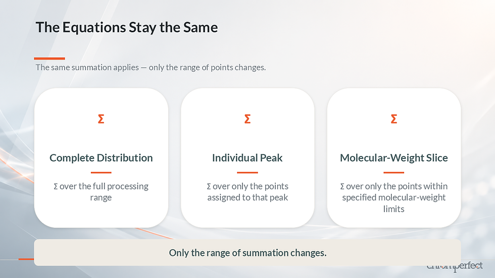
The same molecular-weight equations can be applied to:
The complete SEC distribution
An individual chromatographic peak
A selected molecular-weight slice
The equations remain unchanged.
Only the range of data points included in each summation changes.
For the complete distribution, the summation covers the full SEC processing range.
For an individual peak, it covers only the points assigned to that peak.
For a molecular-weight slice, it covers only the points within the specified molecular-weight limits.
Molecular-weight fractions
In many polymer applications, the proportion of material above or below a specified molecular weight is as important as the overall averages.
Chromperfect calculates five corresponding molecular-weight fractions:
Number fraction, Fn
Weight fraction, Fw
Z fraction, Fz
Z-plus-one fraction, Fz+1
Viscosity fraction, Fv
For each fraction:
The numerator represents the selected point, peak, slice or molecular-weight region.
The denominator represents the complete SEC processing range.
Number, weight, Z and Z-plus-one fractions
The number fraction is:
Fn = Σselected Ai / Σtotal Ai
The weight fraction is:
Fw = Σselected(Ai × Mi) / Σtotal(Ai × Mi)
The Z fraction is:
Fz = Σselected(Ai × Mi²) / Σtotal(Ai × Mi²)
The Z-plus-one fraction is:
Fz+1 = Σselected(Ai × Mi³) / Σtotal(Ai × Mi³)
The viscosity fraction compares the intrinsic-viscosity contribution of the selected range with that of the complete distribution:
Fv = [η]selected / [η]total
When the selected range and the complete processing range are identical:
Fn = Fw = Fz = Fz+1 = Fv = 1.0
All fractions therefore equal 100 percent.
Practical use of molecular-weight fractions
Molecular-weight fractions can describe the amount of material:
Above a high-molecular-weight limit
Below a low-molecular-weight limit
Within a defined molecular-weight slice
Within an individual chromatographic peak
These results help an analyst describe not only the average molecular weight of a polymer, but how much of its distribution lies within or outside ranges associated with:
Product behavior
Processing performance
Material quality
Specification limits

SEC integration with axial correction
When axial correction is active, Chromperfect uses the same molecular-weight-average and fraction equations.
The difference is the value represented by Mi.
Without axial correction, Mi is read directly from the original SEC calibration relationship.
With axial correction, Mi represents the corrected molecular weight assigned to each chromatographic data point.
Axial correction addresses broadening introduced by the chromatographic system and is examined in Part 3 of this series.
SEC results and the Bound file
After SEC integration is complete, the calculated results are stored in the Chromperfect Bound file.
The Bound file contains the processed chromatogram together with the information required to reproduce the analysis, plots and reports.
This may include:
Processed chromatographic data
Method information
SEC Calibration information
Integration results
Molecular-weight averages
Molecular-weight fractions
Intrinsic viscosity
Processing limits
Related calculated values
The resulting information is available for molecular-weight-distribution plots, formatted reports and later review.

The complete SEC integration process
SEC integration is more than measuring the area of a broad chromatographic peak.
Reliable SEC/GPC results depend on a complete chain of analytical decisions:
SEC baseline placement
Treatment of detector noise
Flow-rate stability
Detector linearity
Correct declaration of detector-response type
A suitable SEC calibration
Correct processing-range selection
Appropriate molecular-weight calculations
Every included Raw Data point contributes both a detector-response value and an assigned molecular weight.
Those values are combined to calculate:
Mn
Mw
Mz
Mz+1
Mv
Intrinsic viscosity
Molecular-weight fractions
Results for complete distributions, peaks or selected slices
The reliability of the final result therefore depends on every stage of the SEC integration process.

Continue the SEC/GPC Theory Series
Part 2 continues with SEC calibration theory, including:
The physical meaning of molecular-weight averages
SEC calibration-curve behavior
Narrow-standard calibration
Universal calibration
Intrinsic viscosity
Mark–Houwink relationships
Broad-standard calibration
Read Part 2: [READ PART 2]
Watch Part 2: [WATCH PART 2 VIDEO]
Part 3 covers advanced SEC theory, including:
Molecular-weight-distribution plots
Axial broadening
Axial correction
Calculated molecular-weight traces
Local polydispersity
Preparative fractionation
Read Part 3: [READ PART 3]
Watch Part 3: [WATCH PART 3 VIDEO]

Comments